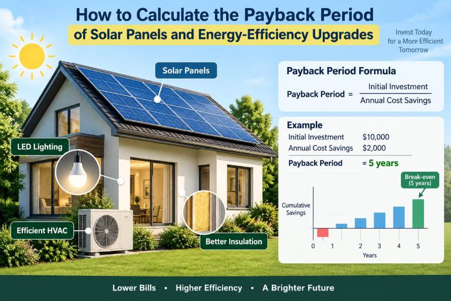

A homeowner receives a quote for rooftop solar, then another for attic insulation, an efficient heat pump, and LED lighting. Every proposal promises lower bills, but the costs arrive today while the savings appear gradually over years. Which project should come first?
A facilities engineer faces a similar decision on a larger scale. Replacing aging motors or improving compressed-air controls may reduce operating costs, yet capital budgets are limited and management wants a clear, defensible answer: when will the project pay for itself?
The payback period offers a practical starting point. It translates an upfront investment into an estimated number of years, months, or billing cycles needed for savings to recover that investment.
Used carefully, payback helps compare solar panels and energy-efficiency upgrades on common ground. Used carelessly, it can hide maintenance costs, changing utility rates, equipment life, and the value that remains after the initial cost has been recovered.
🔎 What the Payback Period Actually Measures
The simple payback period is the time required for cumulative financial savings to equal the project’s net upfront cost. If an upgrade costs $6,000 after incentives and saves $1,000 each year, its simple payback is six years.
It is a screening metric, not a complete financial model. It answers, “How long until I recover my cash outlay?” It does not, by itself, answer whether the project produces the greatest lifetime value.
🧮 The Basic Payback Formula
For savings that are reasonably steady, use:
Simple payback period = Net project cost ÷ Annual savings
Net project cost is the installed price after applicable grants, rebates, tax treatment, or other financial support. Annual savings are the avoided energy costs, minus any new annual costs caused by the project.
For example, a $12,000 solar installation with a $2,000 incentive has a net cost of $10,000. If it avoids $1,250 of electricity purchases per year, the estimated simple payback is eight years.
💰 Start With the True Net Project Cost
The purchase price on a proposal is rarely the complete cost. A useful calculation includes every cost required to put the system into reliable service.
- Equipment, labor, design, permitting, and interconnection charges
- Electrical-panel upgrades, roof work, structural work, or controls integration
- Commissioning, testing, and required inspections
- Financing fees or interest, if you are evaluating financed cash flow
- Expected replacement costs for components with shorter lives, where relevant
Do not subtract an incentive until you understand its eligibility, application process, payment timing, and whether it is based on installed cost, capacity, or measured savings. A potential incentive is not the same as cash already received.
📉 Define Savings as Avoided Cost, Not Just Less Energy
Energy savings are measured in kilowatt-hours, therms, liters of fuel, or another physical unit. Financial savings depend on what those units would have cost. The same 1,000 kWh reduction can be worth very different amounts under different tariffs.
For an electricity-saving measure, a first estimate is:
Annual bill savings = Annual energy reduction × Relevant electricity price
The word relevant matters. A flat residential rate is simple, while a commercial tariff may include time-of-use energy charges, demand charges, fixed charges, and seasonal price differences.
☀️ Estimate Solar Production Before Estimating Savings
Solar panels generate electricity; they do not automatically generate equal bill savings. First estimate annual production in kWh, using a site-specific assessment or reputable modeling tool that accounts for location, tilt, orientation, shading, module rating, and system losses.
Production also changes over time. Modules generally produce somewhat less energy as they age, and unusual weather causes year-to-year variation. For early decisions, use a realistic estimate rather than the sunniest possible year.
A professional design should state important assumptions clearly. If the predicted output is unclear, payback accuracy will be unclear too.
🏠 Match Solar Generation to On-Site Consumption
A solar kWh used immediately in the building often avoids buying a retail-priced kWh. A solar kWh exported to the grid may receive a different credit, depending on local rules and the utility plan.
This is why self-consumption matters: it is the share of solar generation used on site at the time it is produced. Homes empty during sunny afternoons and buildings with low daytime loads may export more electricity than expected.
Review interval consumption data when available. It reveals whether daytime demand aligns with solar output much better than an annual consumption total can.
🧾 Understand Export Credits and Net Billing
Billing arrangements vary widely. Under some structures, exported electricity offsets imported electricity at a similar rate. Under others, exports receive a lower credit, or credits apply only to specific portions of the bill.
Never assume that every generated kWh has the same value as every purchased kWh. Read the tariff, confirm how credits expire or roll over, and ask whether future rate-plan changes could affect the economics.
For a simple annual estimate, separate the value of self-used and exported energy:
Solar savings = Self-used kWh × avoided import rate + Exported kWh × export credit
🕒 Account for Time-of-Use Prices
Time-of-use tariffs charge different prices at different hours. Solar output is strongest around the middle of the day, while a utility’s higher-priced period may occur later in the afternoon or evening.
In that situation, annual solar production alone can overstate bill reduction. Hourly or interval modeling is preferable because it matches generation and load with the price in effect at each time.
A battery, load shifting, or scheduled charging can alter this relationship, but each adds cost and operating assumptions that must be evaluated separately.
🏭 Include Demand Charges for Commercial Facilities
Many commercial and industrial bills include a demand charge based on the highest measured power draw, often in kilowatts, during a billing period. Reducing total kWh does not necessarily reduce that peak.
Solar can lower demand when its output coincides with the facility peak, but clouds, operating schedules, and measurement intervals affect the result. Energy-efficiency measures such as motor controls or cooling improvements may also have limited demand value unless they operate during the peak window.
Do not claim demand-charge savings from a general annual kWh calculation. Use interval data and the actual tariff whenever demand is material.
💡 Calculate Savings From Efficiency Upgrades
Efficiency projects reduce the energy needed to deliver a service: lighting a room, moving air, heating water, or running a production line. Their savings usually begin with a baseline—the energy the existing equipment uses under normal operation.
For a straightforward replacement, estimate:
Annual energy savings = (Old power − New power) × Operating hours
Convert watts to kilowatts before multiplying by hours. Then apply the appropriate energy price. This works well for simple, consistently used equipment, but complex systems need more careful treatment.
💡 Example: LED Lighting Payback
Suppose a building replaces 40 lamps rated at 60 W with 40 LED lamps rated at 10 W. If they operate 3,000 hours annually, the estimated reduction is:
(40 × 0.060 kW − 40 × 0.010 kW) × 3,000 h = 6,000 kWh/year
At an assumed energy value of $0.18 per kWh, that represents $1,080 in annual electricity savings. If the installed project cost is $2,160, the simple energy-only payback is two years.
That hypothetical example may be conservative or optimistic depending on actual hours and rates. It also excludes possible maintenance savings from fewer lamp replacements, which can be meaningful in difficult-to-access spaces.
🌡️ Heating and Cooling Need Seasonal Thinking
Heat pumps, air conditioners, boilers, insulation, and controls do not save a fixed amount every hour. Their consumption depends on weather, setpoints, occupancy, building envelope performance, and part-load operation.
Use seasonal performance information and local operating conditions rather than a nameplate capacity alone. A larger unit is not automatically more efficient in a particular building, especially if poor sizing causes frequent cycling.
For retrofit projects, compare expected annual delivered heating or cooling with the energy required by both the old and new systems. Include auxiliary electric resistance heat, pumps, fans, or fuel use where applicable.
⚙️ Motors, Drives, and Process Loads
Variable-frequency drives can reduce motor energy substantially when a process genuinely needs less flow, pressure, or speed for long periods. They are often strong candidates for fans and pumps, but not every motor load is suitable.
A constant-torque conveyor, for example, may need nearly the same speed whenever it runs. Installing a drive without changing the operating requirement may provide control benefits but modest energy savings.
Measure actual run hours, loading, and control behavior. Electrical measurements and trend data are more reliable than assuming every motor operates at full nameplate power.
🔧 Count Maintenance, Repairs, and Operating Changes
Payback should use net annual savings, not energy savings alone. Some projects reduce maintenance: LEDs may reduce relamping labor, and efficient equipment may have fewer service needs than aging equipment.
Other projects introduce costs. Solar systems may require monitoring, occasional service, insurance considerations, or inverter replacement during their life. Batteries have their own degradation and replacement considerations.
Use this adjusted form:
Net annual savings = Energy savings + Other annual benefits − New annual costs
📊 Use a Cash-Flow Table When Savings Vary
Simple division is inadequate when savings, costs, or incentives change noticeably from year to year. A cumulative cash-flow table shows exactly when the initial outlay is recovered.
| Year | Net cash flow | Cumulative cash flow |
|---|---|---|
| 0 | −$10,000 | −$10,000 |
| 1 | +$1,100 | −$8,900 |
| 2 | +$1,150 | −$7,750 |
| … | … | … |
| 9 | +$1,450 | +$250 |
In this hypothetical case, payback occurs during year 9. If needed, estimate the fraction of that year by dividing the unrecovered balance at the start of the year by that year’s net cash flow.
📈 Know the Difference Between Simple and Discounted Payback
Money available now can be invested, used to avoid borrowing, or reserved for another project. Discounted payback recognizes this time value of money by converting future savings into present-value terms.
Each future cash flow is divided by a factor based on the chosen discount rate and the year in which it occurs. The project pays back when cumulative discounted cash flow becomes positive.
Discounted payback is generally longer than simple payback. It is more realistic for long-lived assets, but its result depends on the selected discount rate, which should reflect the organization’s financial context rather than an arbitrary number.
🧭 Go Beyond Payback With Lifecycle Metrics
A short payback is attractive, but it can favor low-cost projects that stop producing value soon afterward. Two additional measures can make comparisons more complete.
- Net present value (NPV): the present value of future benefits minus present-value costs. A positive NPV at the chosen discount rate indicates value above that required return.
- Internal rate of return (IRR): the discount rate at which NPV becomes zero. It can be useful, though unusual cash-flow patterns can make it misleading.
- Lifecycle cost: the total cost of owning, operating, maintaining, and replacing an asset over a defined study period.
Payback remains valuable for quick screening. Lifecycle measures are better suited to final decisions involving long-lived solar systems, major HVAC equipment, or competing capital projects.
🏦 Treat Financing Separately From Project Economics
A loan, lease, or power-purchase arrangement changes who pays upfront and when. It can improve short-term cash flow, but it does not change how much energy the equipment physically saves.
Evaluate two views: the project economics based on total installed cost and benefits, and the customer cash flow after loan payments, interest, fees, and contract terms. Mixing them can make an expensive financing structure look like a better technical investment than it is.
For third-party solar arrangements, carefully examine escalation clauses, production guarantees, maintenance responsibility, end-of-term options, and property-transfer implications.
🎁 Handle Incentives and Tax Effects Carefully
Rebates, grants, and tax provisions can significantly affect net cost, but their value and timing are not always identical. A rebate may arrive after installation, while a tax benefit may depend on taxable income, ownership structure, and local rules.
For preliminary payback, state whether the incentive is included and when it is expected. For a binding investment decision, confirm eligibility with current program documentation and a qualified tax or financial professional when appropriate.
Avoid treating an incentive as guaranteed merely because it appeared in an advertisement or an old project example.
🔋 Evaluate Batteries as a Separate Decision
A battery can store solar energy for later use, provide backup capability, reduce certain demand peaks, or shift consumption away from expensive periods. Those benefits can be valuable, but they are not free additions to a solar payback calculation.
Model the battery’s installed cost, usable capacity, round-trip losses, cycle limits, control strategy, replacement expectations, and tariff-specific value. Backup power also has a resilience value that may matter greatly to a household or facility even when it does not create the shortest financial payback.
Solar-only and solar-plus-storage should therefore be compared as distinct project cases.
🧱 Recognize Building and Site Constraints
A theoretically efficient improvement can perform poorly if its installation context is ignored. Solar output can be constrained by shading, roof condition, orientation, electrical capacity, and future construction nearby.
Efficiency measures have similar dependencies. Insulation work requires moisture-aware design; ventilation changes must preserve indoor air quality; and HVAC replacements should consider duct leakage, refrigerant piping, controls, and the building envelope.
Addressing these constraints increases upfront scope, but excluding them creates artificially short payback estimates and operational risk.
🧪 Measure the Baseline Before You Promise Savings
The baseline is a representation of energy use before the project. Utility bills are useful, but they may not reveal occupancy changes, production volume, weather differences, or temporary equipment faults.
For larger projects, collect interval electricity data, equipment run hours, maintenance records, and relevant operational data. For weather-sensitive loads, normalize comparisons using appropriate weather information or calibrated models.
Good baseline work does not eliminate uncertainty. It makes the uncertainty visible and reduces the chance of crediting a project for savings caused by unrelated changes.
📏 Use Measurement and Verification After Installation
Measurement and verification, often abbreviated M&V, checks whether expected performance is occurring after installation. The approach can range from reviewing utility bills to submetering equipment and analyzing operational data.
Verification is especially useful when savings are large, performance guarantees exist, or controls changes make outcomes uncertain. It can also uncover simple problems: schedules overridden by staff, failed sensors, panels offline, or equipment operating outside its intended sequence.
Payback estimates should be revisited when measured results materially differ from assumptions.
⚠️ Avoid Common Payback Mistakes
Most weak calculations fail because one assumption is hidden or oversimplified. Watch for these recurring errors:
- Using a headline utility rate while ignoring time-of-use pricing, fixed charges, or export credits
- Assuming every solar kWh offsets a full retail-price purchase
- Using optimistic run hours, sunlight, or occupancy without evidence
- Ignoring maintenance, replacement, permitting, and enabling electrical work
- Comparing a solar project with an efficiency project using different cost assumptions
- Calling a project “paid back” without considering financing obligations or the value of future savings
A transparent estimate with a plausible range is more useful than a precise-looking number built on weak inputs.
🔄 Compare Efficiency First, Solar Second, or Both Together
Efficiency and solar are complementary, but sequence matters. Reducing waste first can lower the solar capacity needed to meet a given portion of consumption, which may reduce capital cost and make electrical infrastructure easier to size.
However, delaying solar solely to complete every possible retrofit may not be sensible if roof work, incentive deadlines, interconnection timing, or organizational priorities favor acting now. The right sequence depends on site conditions and project readiness.
A practical approach is to model at least three cases: efficiency only, solar only, and an integrated efficiency-plus-solar plan. Use consistent energy prices, study periods, and assumptions across all three.
🧱 Consider the Useful Life of Each Asset
Payback should be compared with expected service life. A six-year payback for an asset expected to deliver reliable savings for much longer has a different implication than a six-year payback for equipment nearing replacement.
Solar modules, inverters, HVAC components, lighting drivers, batteries, and controls do not necessarily share the same useful life. Plan for components that may need replacement before the end of the overall project study period.
Also consider the condition of the roof beneath a solar array. Coordinating a needed roof replacement before installation can prevent expensive removal and reinstallation later.
🌦️ Test Sensitivity Instead of Trusting One Scenario
A sensitivity analysis asks how results change when uncertain inputs move. It is one of the best defenses against false confidence.
Test at least a conservative, expected, and favorable case. Vary items such as energy price, annual production, operating hours, self-consumption, maintenance cost, and equipment degradation.
If a project only looks attractive under the favorable case, it deserves additional investigation. If it remains acceptable across reasonable scenarios, the decision is more robust.
🗂️ Build a Practical Calculation Worksheet
A clear worksheet makes review easier and lets assumptions be updated as better information arrives. Keep inputs separate from formulas and document the source of each input.
- Define the project boundary and study period.
- Record installed cost, enabling work, incentives, and expected payment timing.
- Establish baseline energy use and operating conditions.
- Estimate post-project consumption or solar generation.
- Apply tariff-specific avoided costs, export credits, and demand effects.
- Add maintenance changes, replacements, and other annual costs or benefits.
- Calculate simple payback, then evaluate discounted cash flow for major decisions.
- Run sensitivity cases and state the assumptions beside the result.
This process is useful for a home spreadsheet and scales naturally to an industrial capital-approval model.
🧑🔧 Know When to Ask for Professional Help
Simple lighting replacements may be evaluated with basic measurements and bills. Larger projects deserve specialized input when electrical upgrades, structural issues, complex tariffs, financing contracts, process loads, safety requirements, or regulatory obligations are involved.
Qualified installers, energy managers, engineers, and financial advisers serve different roles. Ask technical providers for performance assumptions and design details; ask financial professionals about tax, contract, and ownership implications.
Independent review can be particularly valuable when a proposal presents one attractive payback figure without showing the calculations behind it.
✅ The Core Principle: Compare Honest Cash Flows
Calculating payback is not about finding a single magic number. It is about building an honest connection between an initial investment, the energy behavior it changes, the tariff that converts that change into money, and the costs that continue over time.
For solar, this means modeling production, self-consumption, export value, and system upkeep. For efficiency, it means establishing a credible baseline, realistic operating conditions, and all effects on energy and maintenance.
The best decision is rarely the project with the shortest headline payback alone. It is the project whose benefits, risks, useful life, and cash flows fit the owner’s technical needs and financial constraints.
A trustworthy payback estimate is transparent about its assumptions, cautious about uncertainty, and useful as one part of a broader lifecycle decision. With that foundation, solar and efficiency investments become far easier to compare and improve. ⚡☀️📊