
A rooftop solar array can look perfectly still while its electrical operating conditions change minute by minute. A passing cloud dims part of the array, a breeze cools the modules, and the inverter’s input sees a different voltage-current relationship than it saw moments earlier.
Without active control, a solar panel may produce power, but not its maximum available power. The difference is not merely theoretical: it affects energy harvest, converter loading, battery charging behavior, and the economics of the installation over its lifetime.
Maximum power point tracking, usually shortened to MPPT, is the control process that keeps a photovoltaic system near its best operating point. It is one of the reasons modern solar electronics can adapt effectively to changing sunlight and temperature.
The algorithms behind MPPT range from elegant, low-cost methods used in small chargers to more sophisticated techniques designed for uneven shading and rapidly changing conditions. Understanding their assumptions is the key to selecting, designing, and troubleshooting a system.
☀️ The Electrical Challenge Inside a Solar Panel
A photovoltaic, or PV, cell converts irradiance into electrical current. Many cells are connected into a module, and modules form strings and arrays. Their output is nonlinear: current does not remain proportional to voltage.
At low voltage, a PV module can provide nearly its maximum current. As voltage rises, current stays relatively high for a while, then falls sharply near open-circuit voltage. Because electrical power is voltage multiplied by current, P = V × I, there is one operating region where the product is greatest.
📈 Reading the I–V and P–V Curves
The current-voltage, or I–V, curve shows the output current available at each terminal voltage. The power-voltage, or P–V, curve is derived by multiplying each voltage-current pair.
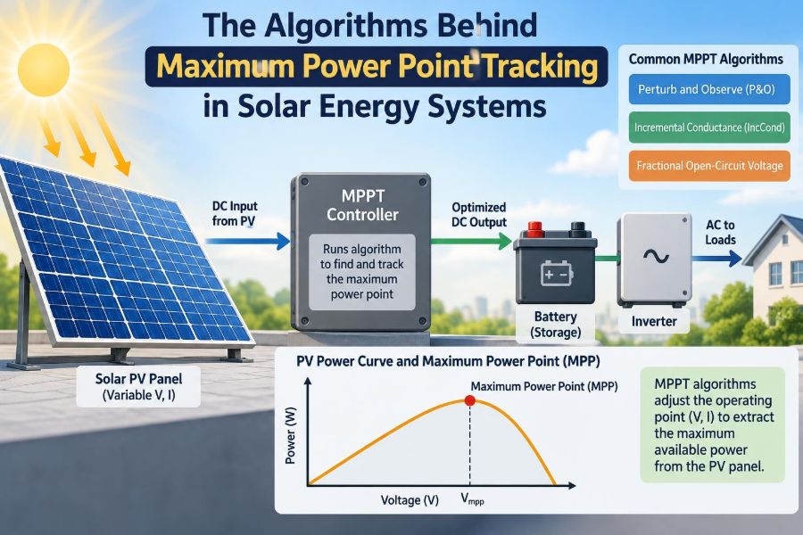
The high point on the P–V curve is the maximum power point (MPP). Its corresponding voltage and current are called Vmp and Imp. An MPPT controller continually seeks this peak rather than locking the panel to one arbitrary voltage.
🔌 Why a Fixed Load Misses Available Energy
A simple resistive load has a fixed relationship between voltage and current. A battery also strongly influences the voltage imposed on a panel, although it is not a fixed resistor. Neither condition will generally match the PV module’s preferred operating point.
Consider a nominal 12 V battery connected directly to a module whose maximum-power voltage is substantially higher under bright conditions. The module is pulled toward the battery voltage, leaving usable voltage and power uncollected. A DC-DC converter lets the input and output operate at different voltages while conserving energy apart from conversion losses.
🔄 The MPPT Control Loop
An MPPT system measures PV voltage and current, calculates or estimates power, and changes a converter command. That command is commonly a duty cycle: the fraction of each switching period for which a transistor is on.
After adjusting duty cycle, the controller observes the new electrical response and decides whether to continue in the same direction or reverse. This closed-loop process repeats continuously, often much faster than ordinary changes in sunlight, though the appropriate rate depends on the converter and sensing system.
⚙️ The Converter Is Part of the Algorithm
MPPT software cannot directly force a solar module to any desired point. It acts through a power converter, typically a buck, boost, buck-boost, or isolated topology. The converter presents an effective input impedance to the PV source.
Changing duty cycle changes that apparent impedance. For example, a buck converter charging a lower-voltage battery can allow a higher-voltage PV input while transferring current to the battery side. Controller design must therefore account for converter dynamics, duty-cycle limits, inductor current behavior, and efficiency.
🧭 What “Tracking” Actually Means
Tracking does not mean measuring a known point once and staying there. Irradiance changes shift the available current, while cell temperature shifts the voltage at which maximum power occurs. Aging, soiling, and mismatch can change the curve as well.
In practice, an MPPT controller makes a tradeoff between speed and stability. It needs to find a moving peak quickly, but it must not create large, wasteful oscillations around that peak or react incorrectly to noise.
👣 Perturb and Observe: The Classic Method
Perturb and Observe, often called P&O or hill climbing, is one of the most widely taught MPPT algorithms. The controller perturbs PV voltage or duty cycle by a small amount and compares the measured power with the previous result.
If power increases, it continues the perturbation in the same direction. If power decreases, it reverses direction. On a smooth, single-peaked P–V curve, this is like walking uphill in fog: take a step, check whether the ground rose, and adjust course accordingly.
✅ Where P&O Works Well
P&O is attractive because it requires only voltage and current measurement, modest computation, and straightforward logic. It performs well in many controllers where irradiance changes relatively slowly compared with the update cycle.
Its simplicity also makes implementation and verification manageable on inexpensive microcontrollers. For an unshaded panel or a well-matched string, it can provide practical performance without a complex mathematical model of the PV array.
⚠️ The Oscillation Problem in P&O
At the peak, any finite perturbation moves the operating point to one side or the other. The controller therefore tends to oscillate around the MPP rather than settle exactly on it. Larger steps find changing peaks faster but produce greater ripple and lost energy near steady state.
A smaller step reduces the steady oscillation but can make tracking sluggish after a sharp change in sunlight. This is a fundamental tuning compromise, not simply a programming error.
🌤️ When Rapid Irradiance Confuses P&O
P&O assumes that a measured power change resulted mainly from its own perturbation. A fast-moving cloud can break that assumption. Power may rise because sunlight increased, even if the controller stepped in the wrong voltage direction.
Practical designs reduce this risk with short measurement intervals, filtered readings, confirmation logic, or adaptive step sizes. No filter should be so slow that it hides real changes; controller timing must match the physical system.
📐 Incremental Conductance and the Slope Rule
The incremental conductance method uses the slope of the P–V curve. Since P = VI, differentiation gives dP/dV = I + V(dI/dV). At maximum power, the slope is zero.
Rearranging yields the condition dI/dV = −I/V at the MPP. To the left of the peak, power rises with voltage; to the right, it falls. The controller estimates changes in current and voltage and uses that relationship to choose its next adjustment.
🧮 Strengths and Costs of Incremental Conductance
Incremental conductance can distinguish a control-induced change from an irradiance-driven change more effectively than basic P&O, particularly when conditions shift quickly. It also has a clear stopping condition near the maximum-power point.
However, numerical differences such as ΔI/ΔV are sensitive to sensor noise, ADC resolution, and small voltage changes. Division can be avoided through cross-multiplication, but careful threshold design is still needed to prevent unstable decisions.
🎯 Constant Voltage Tracking
Constant voltage tracking holds the PV input near a selected fraction of the open-circuit voltage, often based on the observation that maximum-power voltage tends to track open-circuit voltage for a given module family.
This is inexpensive but approximate. Measuring open-circuit voltage may briefly interrupt power transfer, and the preferred fraction changes with temperature, module construction, irradiance, and aging. It suits simple, cost-constrained equipment better than applications demanding the highest possible harvest.
🔋 Constant Current and Battery-Oriented Variants
Some simple designs use a fraction of short-circuit current as an indirect estimate of the MPP. Like constant voltage approaches, this relies on a useful but imperfect PV characteristic.
Battery chargers may also prioritize charge limits, thermal limits, or battery voltage regulation over perfect PV tracking. In that state, the system is intentionally not operating at the PV MPP because accepting all available solar power could violate a battery-management constraint.
🧠 Model-Based and Predictive Approaches
A PV model can estimate the MPP from measured irradiance and temperature, sometimes with periodic correction from electrical measurements. Model-based control can respond rapidly when sensors and parameters are reliable.
Its limitation is parameter drift. Real modules differ from ideal equations, and cable losses, dirt, mismatch, and sensor placement introduce error. Predictive methods are powerful when properly commissioned, but they should retain feedback because the measured array remains the final authority.
🧬 Fuzzy Logic and Neural Approaches
Fuzzy logic controllers express control rules in qualitative terms, such as “if the power slope is slightly positive, increase voltage slowly.” They can handle nonlinear systems without requiring an exact analytical model.
Neural-network and other data-driven approaches can infer complex relationships from training data. Their potential is most relevant where unusual conditions justify extra computation. Their risks include poor behavior outside training conditions, explainability challenges, and a need for disciplined testing rather than faith in algorithm labels.
🌳 Partial Shading Creates Multiple Peaks
Uniform sunlight usually produces one dominant maximum on the array P–V curve. Partial shading is different. A chimney, leaf, snow patch, or nearby structure can reduce current through only part of a string.
Bypass diodes protect shaded cell groups from damaging reverse bias, but they also create steps in the I–V curve. The resulting P–V curve may contain several local maxima. A basic hill-climbing algorithm can stop at a smaller peak even though a higher global maximum exists elsewhere.
🗺️ Local Maxima Versus the Global Maximum
A local maximum is higher than nearby operating points but not necessarily the highest power available across the full voltage range. The global maximum is the best point overall.
This distinction matters most when panels in a series string experience unequal illumination. A controller that tracks perfectly under uniform sunlight may still harvest less energy under recurring partial shade because it is solving the wrong search problem.
🔎 Global MPPT Search Strategies
Global MPPT techniques periodically explore a broader voltage range, identify promising regions, and then use a local tracker for fine control. A voltage sweep is conceptually simple, although sweeping temporarily moves away from the best operating point.
More elaborate methods include particle-based searches, evolutionary searches, and hybrid algorithms. They can locate a global peak under complex shading, but they add computation and tuning choices. The useful question is not whether an algorithm is sophisticated, but whether its added harvest exceeds its complexity and transient losses in the actual site.
🧱 Array Architecture Can Reduce the Problem
MPPT performance is not determined by software alone. Module-level power electronics, such as optimizers or microinverters, allow smaller groups of modules to track independently. This can reduce mismatch losses when roof orientations or shading patterns differ.
Those architectures introduce more electronics, installation considerations, and product-specific service implications. String design, module placement, and avoiding predictable shade often provide a simpler first improvement than asking one central tracker to solve a severely mismatched array.
🌡️ Temperature Moves the Target
Solar modules generally deliver lower voltage as cell temperature rises. A bright summer day can therefore produce high current while shifting the maximum-power voltage below its cool-weather value.
Ambient temperature is not the same as cell temperature. Wind, mounting clearance, irradiance, and roof heat all affect the cells. MPPT responds to the electrical outcome, which is why it remains valuable even when a system has no dedicated temperature sensor.
📏 Sensor Accuracy and Measurement Timing
Every algorithm depends on measured voltage and current. Offset, gain error, switching noise, quantization, and sensor delay can distort the calculated power and slope. A controller may appear to “hunt” because it is responding to measurement artifacts rather than PV behavior.
Voltage and current samples should be synchronized as closely as practical. In a switching converter, sampling at inconsistent points in the switching cycle can create misleading power estimates. Filtering must suppress ripple without adding excessive delay.
⏱️ Sampling Rate, Bandwidth, and Stability
A faster MPPT update is not automatically better. The power stage needs time to respond after a duty-cycle change, and a measurement taken too soon may reflect transient inductor or capacitor behavior rather than the new steady operating point.
A well-designed controller coordinates three time scales: high-frequency converter switching, the converter’s control-loop response, and the slower MPPT search loop. Treating MPPT as independent of voltage and current control loops can create interaction and instability.
🛡️ Operating Limits Override Maximum Power
PV input voltage and current must remain within ratings for transistors, capacitors, inductors, connectors, and insulation. A controller must also respect battery charge limits, inverter DC-link constraints, and thermal conditions.
During curtailment, overload, or a full battery, the correct behavior may be to move away from the MPP. Maximum power point tracking is a subordinate objective: safe and stable operation has priority.
🔥 Converter Efficiency Changes the Real Result
MPPT maximizes power drawn from the panel, but system designers care about useful power delivered to the battery, load, or grid interface. Conduction loss, switching loss, magnetic loss, and control consumption reduce that output.
An aggressive algorithm that makes the converter move frequently can add ripple and switching-related loss. Evaluating only PV-side power can therefore hide a poor system-level tradeoff. Input tracking and output efficiency should be assessed together.
🧪 A Practical Design Workflow
Start with the PV array’s expected voltage and current range, including cold open-circuit voltage and hot operating voltage. Then select a converter topology that can meet output requirements without violating component ratings.
- Characterize the intended array, battery, or DC bus and expected shading conditions.
- Choose sensing hardware and establish realistic noise and resolution limits.
- Implement baseline protection and stable converter control before enabling MPPT.
- Select an algorithm that matches the operating environment.
- Test steady sunlight, irradiance steps, temperature changes, and shaded-array cases.
- Log voltage, current, power, duty cycle, temperatures, and fault states for diagnosis.
🧰 Choosing an Algorithm by Application
| Application condition | Often suitable starting approach | Key caution |
|---|---|---|
| Small, low-cost charger | Constant-voltage or basic P&O | Approximation may leave energy unused |
| Uniformly illuminated array | P&O or incremental conductance | Tune step size and filtering |
| Rapidly changing sunlight | Incremental conductance or adaptive P&O | Verify sensor timing and noise immunity |
| Frequent partial shading | Local tracker plus periodic global search | Account for scan losses and multiple peaks |
| Complex module mismatch | Improved array architecture or module-level tracking | Compare lifecycle complexity, not just algorithm capability |
This table is a starting point, not a universal prescription. Hardware topology, firmware resources, safety requirements, and site conditions can change the best choice.
🚫 Common MPPT Implementation Mistakes
- Using the wrong control direction: duty cycle and PV voltage do not move in the same direction for every converter topology.
- Ignoring converter settling: comparing transient readings leads to false tracking decisions.
- Using one fixed perturbation step: it often performs poorly in both calm and rapidly changing conditions.
- Assuming one peak: partial shading can invalidate this assumption.
- Testing only with a bench supply: a stiff supply does not reproduce the nonlinear PV curve.
- Forgetting fault behavior: startup, disconnects, overvoltage, and sensor failures need defined responses.
📊 Testing With Realistic PV Conditions
A programmable PV emulator is useful because it can reproduce I–V curves, irradiance steps, and multiple peaks repeatably. Outdoor tests are equally valuable because they reveal thermal behavior, noise coupling, and conditions that models may miss.
Compare algorithms by observing settling time, oscillation near the peak, behavior after irradiance changes, global-peak detection under representative shade, and delivered output energy. A single instantaneous efficiency number rarely describes the full operating experience.
🔧 Field Diagnostics When Harvest Looks Low
Low solar output does not automatically mean an MPPT fault. Check irradiance, soiling, shade, module orientation, string configuration, connection resistance, inverter limits, battery state, and temperature before blaming the algorithm.
Useful logs show PV voltage, PV current, calculated power, output power, duty cycle, and status flags over time. If PV voltage is persistently far from the expected MPP region when the downstream system can accept power, the tracker or its measurements deserve closer inspection.
🔐 Reliability and Fail-Safe Behavior
Controllers should handle implausible sensor values, loss of communication, startup with low irradiance, reverse polarity where relevant, and abrupt load disconnection. Firmware should define safe duty-cycle limits rather than allowing an arithmetic fault to command an unsafe state.
Robust designs also avoid relying on a single perfect measurement. Plausibility checks, watchdogs, current limits, thermal derating, and orderly restart logic turn an MPPT algorithm into a dependable power-management system.
🌍 The System-Level Value of Better Tracking
Improved tracking can increase energy capture when a system frequently operates away from its natural maximum-power point. The value depends on local weather, array configuration, shading, conversion efficiency, and what the load can accept.
There is no universal gain attributable to MPPT because the baseline and conditions vary widely. Engineers should estimate value using site-specific energy behavior, not assume that a more advanced controller automatically produces a proportionate benefit.
🧩 The Core Principle to Remember
MPPT is an optimization problem embedded in a real power converter. The PV array supplies a changing nonlinear source, sensors provide imperfect observations, and the converter can only move within physical and safety limits.
The best implementation matches the algorithm to the curve it must track. Basic P&O may be entirely appropriate for a stable, unshaded system; incremental conductance can improve response to changing irradiance; and global-search methods become relevant when partial shading creates multiple peaks.
Most importantly, good MPPT is not a contest to use the most complicated algorithm. It is the disciplined combination of a suitable converter, credible measurements, stable control loops, sensible protection, and testing under the conditions the equipment will actually face.
Maximum power point tracking succeeds when the controller continuously turns changing solar conditions into the best safe operating point for the entire electrical system. That is the practical engineering idea behind every well-designed solar tracker. ☀️⚡🔋