Aperiodic Signal Representation by Fourier Integral
An aperiodic function will never repeat, although technically speaking an aperiodic function can be considered similar to a periodic function with an infinite period. In order to show that an aperiodic signal can be expressed as a continuous sum (or integral) of infinite exponentials, a limiting process is applied. In order to represent an aperiodic signal f(t), such as the signal shown in Fig. 1.1a by infinite exponential signals, a new periodic signal
fT0fT0
must be formed by repeating the aperiodic signal f(t) every T0 seconds, shown in Fig. 1.1b. The period is made just long enough to not overlap between each repeating pulse. This periodic signal
fT0fT0
is represented by an exponential Fourier series. By letting
T0→∞T0→∞
, the pulses in the periodic signal repeat themselves after an infinite interval, therefore:
limT0→∞fT0(t)=f(t)limT0→∞fT0(t)=f(t)
The Fourier series representing
fT0fT0
will thus also represent f(t) in the limit
T0→∞T0→∞
. The exponential Fourier series can be represented for
fT0fT0
as follows
fT0(t)=∑n=−∞∞Dnejnω0tfT0(t)=∑n=−∞∞Dnejnω0t
(1.1)
by which
Dn=1T0∫T02−T02fT0(t)e−jnω0tdtDn=1T0∫−T02T02fT0(t)e−jnω0tdt
(1.2a)
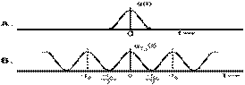
FIGURE 1.1. Construction of a periodic signal by periodic extension of f(t)
Figure 1.1 represents the construction of a periodic signal by periodic extension of f(t)
and
ω0=2πT0ω0=2πT0
(1.2b)
Figure 1.1a and 1.1b show that integrating
fT0fT0
over
−T02,T02−T02,T02
is exactly the same as if you were to integrate over
(−∞,∞)(−∞,∞)
. Simplifying the integration bounds, Eq 3.2a is now expressed by
Dn=1T0∫∞−∞fT0(t)e−jnω0tdtDn=1T0∫−∞∞fT0(t)e−jnω0tdt
(1.2c)
An interesting phenomenon is that the spectrum changes at T0 increases. To better understand this odd behavior,
F(ω)F(ω)
is defined as a continuous function of
ωω
, as
F(ω)=∫∞−∞f(t)e−jωtdtF(ω)=∫−∞∞f(t)e−jωtdt
(1.3)
The last two equations above show that
Dn=1T0F(nω0)Dn=1T0F(nω0)
(1.4)
What this shows is that the Fourier coefficients Dn are (1/T0 times) the samples of
F(ω)F(ω)
spaced uniformly at intervals of
ω0ω0
rad/s, as shown in Fig. 1.2a. For simplicity, Dn and
F(ω)F(ω)
are assumed to be real in Fig. 1.2. Letting
T0→∞T0→∞
by doubling T0 repeatedly, halves the fundamental frequency
ω0ω0
; this operation is used so that there are twice as many components (or samples) in the spectrum. Consequently, by doubling T0 , the envelope
(1T0)F(ω)(1T0)F(ω)
is halved, shown in Fig 1.2b. If T0 is doubled over and over again, the spectrum will become denser while its magnitude becomes smaller. Nothing that in the limits
T0→∞T0→∞
,
ω0→∞ω0→∞
, and
Dn→∞Dn→∞
, the relative shape of the envelope is kept the same. This means that the spectrum must be so dense that the spectral components are spaced at zero (or infinitesimal) level! Simultaneously, the amplitude of each component is also zero. This may seem peculiar at first glance; however, it will be shown that these are classic characteristics of a very familiar phenomenon. By substituting Eq. 1.4 in Eq. 1.1, the following sum yields
fT0(t)=∑n=−∞∞F(nω0)T0ejnω0fT0(t)=∑n=−∞∞F(nω0)T0ejnω0
(1.5)
Here as
T0→∞T0→∞
,
ω0ω0
becomes extremely small
(ω0→0)(ω0→0)
. Due to this limit, a more appropriate notation will replace
ω0ω0
,
ΔωΔω
. With this new notion, Eq. 1.2b is now written as
Δω=2πT0Δω=2πT0
and Eq. 1.5 is now written as
fT0(t)=∑n=−∞∞[F(nΔω)Δω2π]e()jnΔω)tfT0(t)=∑n=−∞∞[F(nΔω)Δω2π]e()jnΔω)t
(1.6a)
Here, Eq. 1.6a shows that
fT0(t))fT0(t))
may be expressed in terms of a sum of infinite exponentials with frequencies
0,±Δω,±2Δω,±3Δω,…0,±Δω,±2Δω,±3Δω,…
, which is the Fourier series. In the limit as
T0→∞T0→∞
,
ω0→∞ω0→∞
, and
Dn→∞Dn→∞
, the amount of the component of frequency
nΔωnΔω
is
[F(nΔω)Δω]/2π[F(nΔω)Δω]/2π
. Thus,
f(t)=limT0→∞fT0(t)=limΔω→012π∑n=−∞∞F(nΔω)e(njΔω)tΔωf(t)=limT0→∞fT0(t)=limΔω→012π∑n=−∞∞F(nΔω)e(njΔω)tΔω
(1.6b)
On the right side of Eq 1.6b, the sum is the area under the function
F(ω)ejωtF(ω)ejωt
, as shown in Fig. 1.3. Thus,
f(t)=12π∫∞−∞F(ω)ejωtdωf(t)=12π∫−∞∞F(ω)ejωtdω
(1.7)
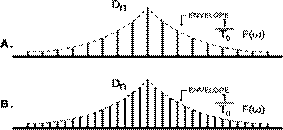
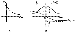
FIGURE 1.2 Change in the Fourier spectrum when the period T0 in Fig 1.1 doubles.
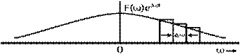
FIGURE 1.3 The Fourier series becomes the Fourier integral in the limit as
T0→∞T0→∞
The integral on the right side is known as the Fourier integral. This is the representation of an aperiodic signal f(t) by a Fourier integral, rather than a Fourier series. This Fourier integral is essentially a Fourier series (only in the limit) with fundamental frequency
Δω→0Δω→0
, as shown in Eq. 1.6.
Assigning
F(ω)F(ω)
as the direct Fourier transform of f(t), and f(t) as the inverse Fourier transform of
F(ω)F(ω)
. Another way to convey this statement is by a Fourier transform pair as stated below
F(ω)=F[f(t)] and f(t)=F[F(ω)]F(ω)=F[f(t)] and f(t)=F[F(ω)]
or
f(t)⇔F(ω)f(t)⇔F(ω)
To summarize,
F(t)=∫∞−∞f(ω)ejωtdωF(t)=∫−∞∞f(ω)ejωtdω
(1.8a)
and
f(t)=12π∫∞−∞F(ω)ejωtdωf(t)=12π∫−∞∞F(ω)ejωtdω
(1.8b)
The spectrum of
F(ω)F(ω)
can also be plotted as a function of
ωω
. Because
F(ω)F(ω)
is complex, both the amplitude and angle spectra are as follows:
F(ω)=|F(ω)|ejθ0(ω)F(ω)=|F(ω)|ejθ0(ω)
Conjugate Symmetry Property
From Eq. 1.8a, if f(t) is a real function of t, then
F(ω)F(ω)
and
F(−ω)F(−ω)
are known to be complex conjugates shown below.
F(−ω)=F∗(ω)F(−ω)=F∗(ω)
(1.9)
Therefore,
|F(−ω)|=|F(ω)||F(−ω)|=|F(ω)|
(1.10a)
θf(−ω)=−θf(ω)θf(−ω)=−θf(ω)
(1.10b)
Consequently, for real f(t), the amplitude spectrum
|F(ω)||F(ω)|
is an even function, and the phase spectrum
θf(ω)θf(ω)
is an odd function of
ωω
. Only for real f(t), this property known as the conjugate symmetry property holds true. This transform of
F(ω)F(ω)
is the frequency domain specification of f(t).
Example
Find the Fourier transform of
e−atu(t)e−atu(t)
By definition of Eq. 1.8a,
F(ω)=∫∞−∞e−jωtdt=∫∞0e−(a+jω)tdt=−1a+jωe(a+jω)t|∞0F(ω)=∫−∞∞e−jωtdt=∫0∞e−(a+jω)tdt=−1a+jωe(a+jω)t|0∞
But
∣∣e−jωt∣∣=1|e−jωt|=1
. Therefore, as
t→∞,e−(a+jω)t=e−ate−jωt=0t→∞,e−(a+jω)t=e−ate−jωt=0
if
a>0a>0
. Therefore,
F(ω)=1a+jω a>0F(ω)=1a+jω a>0
Existence of the Fourier Transform
In the above example, it was shown that when a < 0, the Fourier integral for
e−atu(t)e−atu(t)
does not converge. Thus, the Fourier transform for
e−atu(t)e−atu(t)
does not exist if a < 0 (that is, exponentially growing). Observing from this example, not all signals are transformable. Any existence of the Fourier transform is assured for any f(t) that satisfies the Dirichlet conditions. The first of the conditions is as follows
∫∞−∞|f(t)|<∞∫−∞∞|f(t)|<∞
(1.12)
In order to show this holds true, recall that
∣∣e−jωt∣∣=1|e−jωt|=1
. Thus from Eq. 1.8a,
|F(ω)|≤∫∞−∞|f(t)|dt|F(ω)|≤∫−∞∞|f(t)|dt
By expressing
a+jωa+jω
in the polar form as
a2+ω2−−−−−−√ejtan−1(ωa)a2+ω2ejtan−1(ωa)
,
F(ω)=1a2+ω2−−−−−−√e−jtan−1(ωa)F(ω)=1a2+ω2e−jtan−1(ωa)
Therefore
|F(ω)|=1a2+ω2−−−−−−√|F(ω)|=1a2+ω2
and
θf(ω)=−tan−1(ωa)θf(ω)=−tan−1(ωa)
The amplitude spectrum of
|F(ω)||F(ω)|
and the phase spectrum
θf(ω)θf(ω)
are shown in Figure 1.4b. Observe that
|F(ω)||F(ω)|
is an even function of
ωω
, and
θf(ω)θf(ω)
is an odd function of
ωω
, as expected to be.
As long as condition 1.12 is satisfied, it shows that the existence of the Fourier transform is assured.
Linearity of the Fourier Transform
The Fourier transform can be considered linear if
f1(t)⇔F1(ω)f1(t)⇔F1(ω)
and
f2(t)⇔F2(ω)f2(t)⇔F2(ω)
then,
a1f1(t)+a2f2(t)⇔a1F1(ω)+a2F2(ω)a1f1(t)+a2f2(t)⇔a1F1(ω)+a2F2(ω)
(1.13)
This result can be extended to any finite number of terms. This proof is trivial and follows exactly from Eq. 1.8a.
Coming Up
As of now, you should have an understanding of what an aperiodic signal is and how it is represented by a Fourier Integral. By applying a limiting process, you should know how an aperiodic signal can be expressed as a continuous sum over everlasting exponentials, how the linearity of the Fourier Transform proof is satisfied, and how to find a Fourier transform using its spectra as well as the conjugate symmetry property. Next, an understanding of some useful functions, signal bandwidth, filtering (or interpolating), as well as the synthesis of a time-limited pulse signal.